Simple Linear Regression using TensorFlow 2

Simple linear regression is a statistical method that is used to analyze the relationship between two continuous variables:

• x - independent variable also known as explanatory or predictor.
• y - dependent variable also known as response or outcome.

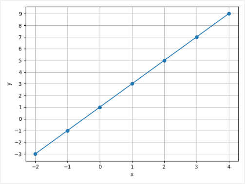
Let's say we have the following sets of numbers:

You may notice that the x value is increasing by 1, and the corresponding y value is increasing by 2. So relationship is y = 2 * x + 1.

This tutorial provides an example how to create and train a model which predicts the value of y for the given value of x. We will use TensorFlow 2.

Using pip package manager, install tensorflow from the command line.

pip install tensorflow

We declare arrays of x and y values which will be used to train the model. The model has one layer which has one neuron. An input shape to it is only composed of one value. The model is compiled by using two arguments - a loss function and an optimizer.

A loss function quantifies the error between the output of the model (predicted value) and a given target value (expected value). A loss function, sometimes called an error function. We use mean squared error (MSE) for the loss function.

An optimizer updates the weights of the model in response to the output of the loss function. An optimizer goal is to minimize the loss function. We use stochastic gradient descent (SGD) for the optimizer.

from tensorflow import keras
import numpy as np

xs = np.array([-2.0, -1.0, 0.0, 1.0, 2.0, 3.0, 4.0], dtype=float)
ys = np.array([-3.0, -1.0, 1.0, 3.0, 5.0, 7.0, 9.0], dtype=float)

model = keras.Sequential([
    keras.layers.Dense(units=1, input_shape=[1])
])

model.compile(optimizer='sgd', loss='mean_squared_error')

model.fit(xs, ys, epochs=400)

x = 15.0
y = model.predict([x])
print(y[0])

The fit method is used to train the model. It learns the relationship between the values of x and y. Training process is used to minimize the loss function using the optimizer. The number of epochs defines how many times the learning algorithm will go over the entire x and y data provided. We use 400 epochs.

At beginning, a value of the loss function is quite large, but it becomes smaller on each epoch.

Epoch 1/400
1/1 [==============================] - 0s 0s/step - loss: 51.6037
Epoch 2/400
1/1 [==============================] - 0s 0s/step - loss: 41.3722
Epoch 3/400
1/1 [==============================] - 0s 0s/step - loss: 33.1710
..................

Ending of the training, a value of the loss function is very small. It means that model learned the relationship between the values of x and y.

..................
Epoch 398/400
1/1 [==============================] - 0s 0s/step - loss: 3.0841e-07
Epoch 399/400
1/1 [==============================] - 0s 0s/step - loss: 2.9904e-07
Epoch 400/400
1/1 [==============================] - 0s 0s/step - loss: 2.8995e-07

We can use the trained model to predict a value of y for a previously unknown value of x.

In this case, if x is 15.0, then the model returns that y is 31.004467. We can verify by calculating:

y = 2 * x + 1 = 2 * 15 + 1 = 31