CIFAR-10 is a dataset that consists of 60000 color images. The dataset is divided into 50000 training images and 10000 testing images. Each image is a 32x32 size, associated with a label from 10 classes. There are 6000 images in each class.
| Label | Class name |
|---|---|
| 0 | Airplane |
| 1 | Automobile |
| 2 | Bird |
| 3 | Cat |
| 4 | Deer |
| 5 | Dog |
| 6 | Frog |
| 7 | Horse |
| 8 | Ship |
| 9 | Truck |
This tutorial provides example how to use convolutional neural network (CNN) to classify CIFAR-10 images. We will use TensorFlow 2.
Using pip package manager, install tensorflow from the command line.
pip install tensorflowTensorFlow 2 provides the ready to use CIFAR-10 dataset, which can be loaded by using the load_data function. It downloads the dataset and caches it on the filesystem. To verify that the dataset loaded successfully, we will display a few images.
plot.py
from tensorflow import keras
import matplotlib.pyplot as plt

classNames = ['airplane', 'automobile', 'bird', 'cat', 'deer',
              'dog', 'frog', 'horse', 'ship', 'truck']

cifar10 = keras.datasets.cifar10
(trainImages, trainLabels), (testImages, testLabels) = cifar10.load_data()

fig, ax = plt.subplots(1, 10)
for i in range(0, 10):
    ax[i].axis('off')
    ax[i].set_title(classNames[testLabels[i][0]])
    ax[i].imshow(testImages[i])

plt.show()
We display the first 10 testing images.

The load_data function returns sets of training and testing images with associated labels. We apply normalization on each set by dividing each pixel value by 255 to get a range of 0 to 1. It improves activation functions performance.
We build a convolutional neural network by stacking the Conv2D and MaxPooling2D layers. The shape of input is [32, 32, 3]. It corresponds to [image_height, image_width, color_channels]. CIFAR-10 has 10 classes, so the last layer has 10 outputs.
The model is compiled using sparse categorical cross-entropy loss function and Adam optimizer. We use the metrics parameter to report the accuracy of the training.
We use 10 epochs to train the model. The validation_data parameter defines data which will be used to evaluate the loss and accuracy at the end of each epoch. The model will not be trained on this data. We don't have a separate validation set, so we use the testing set.
train.py
from tensorflow import keras
from matplotlib import pyplot as plt

cifar10 = keras.datasets.cifar10
(trainImages, trainLabels), (testImages, testLabels) = cifar10.load_data()

trainImages = trainImages / 255
testImages = testImages / 255

model = keras.Sequential([
    keras.layers.Conv2D(32, (3, 3), activation='relu', input_shape=(32, 32, 3)),
    keras.layers.MaxPooling2D((2, 2)),
    keras.layers.Conv2D(128, (3, 3), activation='relu'),
    keras.layers.MaxPooling2D((2, 2)),
    keras.layers.Conv2D(64, (3, 3), activation='relu'),
    keras.layers.Flatten(),
    keras.layers.Dense(128, activation='relu'),
    keras.layers.Dense(10, activation='softmax')
])

model.compile(
    optimizer='adam',
    loss='sparse_categorical_crossentropy',
    metrics=['accuracy']
)

trainHistory = model.fit(
    trainImages,
    trainLabels,
    epochs=10,
    validation_data=(testImages, testLabels)
)

plt.plot(trainHistory.history['accuracy'])
plt.plot(trainHistory.history['val_accuracy'])
plt.ylabel('Accuracy')
plt.xlabel('Epoch')
plt.legend(['Training', 'Validation'])
plt.grid()
plt.show()

(loss, accuracy) = model.evaluate(testImages, testLabels)
print(loss)
print(accuracy)

model.save('model.h5')
We display the training history. It shows accuracy on the training and validation sets for each epoch.
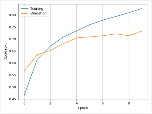
We evaluate the model by using a testing set. In this case, we got an accuracy of 0.7333. It means that model accuracy is about 73%.
0.852361798286438
0.733299970626831
Trained model is saved in HDF5 format.
A model was trained, and now we can predict classes for the given images.
test.py
import tensorflow as tf
from tensorflow import keras
from matplotlib import pyplot as plt

classNames = ['airplane', 'automobile', 'bird', 'cat', 'deer',
              'dog', 'frog', 'horse', 'ship', 'truck']

cifar10 = keras.datasets.cifar10
(trainImages, trainLabels), (testImages, testLabels) = cifar10.load_data()

testImages = testImages / 255

model = keras.models.load_model('model.h5')

classifications = model.predict(testImages[:10])

fig, ax = plt.subplots(1, 10)
for i in range(0, 10):
    predictedLabel = tf.math.argmax(classifications[i])

    ax[i].axis('off')
    ax[i].set_title(classNames[predictedLabel])
    ax[i].imshow(testImages[i])

plt.show()
We predict classes for the first 10 testing images. A model incorrectly predicted class for the third image.





Leave a Comment
Cancel reply